Capital One Labs Financial Data Modelling
One primary interest of financial companies is to model customer risk. For credit cards, this risk can be represented as a metric related to credit score. This score is used to determine credibility - often for credit card application approval, and credit limit.
With massive data collection in today's world, there is often an overabundance of features. This means some information can be redundant and depending on what questions you are asking - is useless. Therefore, it is of interest to reduce the dimensionality by applying feature reduction. One primary advantage of this is to lower model size, and therefore improve speed and scalability of modeling to arrive at actionable insight more quickly.
In this project, I applied machine learning algorithms to Capital One financial data with the goal of predicting a value linked to credit score. The training set consists of approximately 5000 records, each containing 254 features, and one "target" column, representing the desired prediction to train. This analysis is an excellent example of feature reduction, and demonstrates backwards stepwise selection and best subset selection.
The data for this project can be found at this address. One of the first things to notice is the features of the dataset. Most of them are numerical, but there are some which are categorial. A summary of those features is as follows:
target = y_values (to predict)
f_237 = Countries (USA, Mexico, Canada)
f_215 = Status/Color (red, orange, yellow, blue)
f_61 = single lowercase grade(a, b, c, d, e)
f_121 = single uppercase grade (A, B, C, D, E, F)
In order to use these for regression type modeling, the text will need to be encoded and transformed. We'll start by importing some libraries, setting up a text data frame to use with DictVectorizer() from SciKitLearn.
import pandas as pd
import numpy as np
import matplotlib.pyplot as plt
from scipy.stats import norm
from itertools import combinations
import dill as pickle
from sklearn.linear_model import LinearRegression, Ridge
from sklearn import cross_validation, preprocessing, svm
from sklearn.feature_extraction import DictVectorizer
from sklearn.grid_search import GridSearchCV
from sklearn.decomposition import PCA
from sklearn.pipeline import Pipeline
#read training and test data and drop rows which have NaN in the text columns. We can impute the rest of the numerical NaN data.
df_train = pd.read_table('codetest_train.txt', sep='\t')
df_test = pd.read_table('codetest_test.txt', sep='\t')
df_train = df_train.dropna(subset=['f_237', 'f_215', 'f_61', 'f_121'])
df_test = df_test.dropna(subset=['f_237', 'f_215', 'f_61', 'f_121'])
# 4632 rows after NaN drop
#create text data frames to vectorize
df_text = df_train[['f_237', 'f_215', 'f_61', 'f_121']]
df_text_test = df_test[['f_237', 'f_215', 'f_61', 'f_121']]
#vectorize data from array using fit_transform, and place vectorized binary values into dataframe
DV = DictVectorizer(sparse=False)
category_dict = df_text.T.to_dict().values()
category_dict_test = df_text_test.T.to_dict().values()
vect_text = DV.fit_transform(category_dict)
vect_text_test = DV.transform(category_dict_test)
df_vecttext = pd.DataFrame(vect_text)
df_vecttext_test = pd.DataFrame(vect_text_test)
#reindex, cast as float, and merge with original data frame.
df_train = df_train.reset_index(drop=True)
df_vecttext.astype(float)
df_train = pd.concat((df_vecttext, df_train), axis=1)
df_test = df_test.reset_index(drop=True)
df_vecttext_test.astype(float)
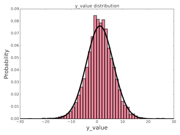
df_test = pd.concat((df_vecttext_test, df_test), axis=1)Next, we can setup the "target" values (y) for modeling. It's always interesting just to look at the data you are trying to predict. There could be some easily identifiable patterns which can tell you something general about the data. We can view the distribution of "target" values as a histogram, and (*gasp*) it appears to be a simple gaussian distribution! (I'll leave it to you to figure out how to set this up using Matplotlib, it's easy.
#now setup arrays for modeling and drop text data and "target" from original data frames, as the vectorized versions are now present.
y_train = df_train['target'].values
y = df_train['target'].values
cc_df = df_train.drop(['f_237', 'f_215', 'f_61', 'f_121'], 1)
df_train = df_train.drop(['target', 'f_237', 'f_215', 'f_61', 'f_121'], 1)
df_test = df_test.drop(['f_237', 'f_215', 'f_61', 'f_121'], 1)
Now with the data cleaned, vectorized, and structured, we can begin to start our modeling. The best place to start can often be one of the simplest things to do - a basic linear model. In this model, we assume our features are all linearly correlated to our target value, and can feed them directly into a linear type regression. One last step we'll need to do is to impute the missing values for the fields which are missing data. This can be done using SciKitLearn's Imputer().
#convert x values to array and impute the NaN values using averages along columns
x_training = np.array(df_train)
x_testing = np.array(df_test)
imputer = preprocessing.Imputer(missing_values='NaN', strategy='mean', axis=0)
x_training = imputer.fit_transform(x_training)
x_testing = imputer.transform(x_testing)

#initialize regressor, setup cross-validation, perform fit
LR = LinearRegression()
test_set = 0.2 #20% is a good testing set that often yields the lowest out of sample error
cv = cross_validation.ShuffleSplit(len(y_train), n_iter=10, test_size=test_set, random_state=42)
AccScore_linear = cross_validation.cross_val_score(LR, x_training, y_train, cv=cv)
print "Full Linear Regression Model = ", ("Accuracy: %0.3f (+/- %0.3f)" % (AccScore_linear.mean(), AccScore_linear.std() * 2))
As you can see, the prediction accuracy is not spectacular. We cannot change the data (it speaks for itself!), but there may be some tricks we can try to reduce the model size. One of these could be to use a linear_model.Lasso() regression and apply a gridsearch cv over the alpha parameter. We could also use PCA, but generally the fit is always best with all of the data - anything less results in poorer predictions. Yet another option would be to take a stepwise approach to determining which features contribute the most to the prediction value. This can be used to apply backwards and forwards feature selection. To do this we will use the Pandas library, as it has some nice functions.
We can start by calculating the Pearson correlation coefficients for each of the features and the "target" values. From here, we can use only the ones which are most strongly correlated, thereby significantly reducing model size.
#setup an iterable for CC values, calculate CC values over the iterable, and plot resulting values as a histogram
            columnlist = cc_df.columns.tolist()
columnlist = [str(item) for item in columnlist]
cc_df.columns = columnlist
CC_target = [cc_df[columnlist[i]].corr(cc_df['target']) for i in range(0,len(columnlist))]

NUM_COLORS = len(CC_target) #determine number of colors
fig = plt.figure()
cm = plt.get_cmap('gist_rainbow')
ax = fig.add_subplot(111)
ax.set_color_cycle([cm(1.*i/NUM_COLORS) for i in range(NUM_COLORS)]) #setup a color cycle
colors = [cm(1.*(i)/NUM_COLORS) for i in range(1,NUM_COLORS+1)]
nx = np.array(range(NUM_COLORS))
ny = np.array(CC_target)
ny = ny.tolist()
ny = np.array(ny)
width = 1/1.5 #set width of bars
inds = ny.argsort() #sort by the cc values
ny = np.sort(ny) #sort y
columnlist = np.array(columnlist)[inds] #use sort for x labels
colors = np.array(colors)

for i in range(0,len(CC_target)):
    plt.bar(nx[i], ny[i], width, color=colors[i], align='center', edgecolor='k', lw=1)

plt.xticks(nx, columnlist, rotation=45, ha='right', fontsize=12)
plt.ylabel('Correlation coefficient (target vs features)', fontsize=12)
plt.tight_layout()
plt.savefig('CC_target_vs_features', dpi=300)
plt.clf()
plt.show()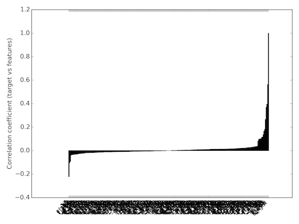
It is a bit difficult to see the x-axis labels, but it is not important. Here I have ranked the histogram by the CC values from low to high. While there are a few features which are strongly positively and negatively correlated with the "target" values, most are not. Let's select only those which are greater or less than an absolute CC value and feed them into another linear model.
indices = np.array(CC_target).argsort()
cc_features = np.sort(np.array(CC_target)).tolist()

reduced_features = []
reduced_labels = []

neg_corr_features = []
neg_corr_featurelabels = []
#loop for reduction

for i in range(0,len(columnlist)):
    #the values given represent the best cut-offs for feature selection, based on analysis of the resulting linear regression model output
    if cc_features[i] > float(0.08):
        reduced_features.append(cc_features[i])
        reduced_labels.append(columnlist[i])

    elif cc_features[i] < float(-0.04):
        reduced_features.append(cc_features[i])
        reduced_labels.append(columnlist[i])
        neg_corr_features.append(cc_features[i])
        neg_corr_featurelabels.append(columnlist[i])

#now setup reduced data frames and convert to arrays for fitting
print reduced_labels
iterable_list = list(cc_df.columns)
iterable_list.remove('target')
#print reduced_labels
cc_df = cc_df[reduced_labels]
cc_df = cc_df.drop('target', 1)
#cc_test_df = df_test[reduced_labels]

#setup x arrays for fitting
x_train1 = np.array(cc_df)
x_train1 = imputer.fit_transform(x_train1)

#remember x_testing is the test df
reduced_labels.remove('target')
AccScore_linear_reduced = cross_validation.cross_val_score(LR, x_train1, y_train, cv=cv)
print "Reduced Linear Regression Score = ", ("Accuracy: %0.3f (+/- %0.3f)" % (AccScore_linear_reduced.mean(), AccScore_linear_reduced.std() * 2))
#so the reduced feature dataset gives a better prediction!
So, it seems this reduced model gives just as good of a prediction, if not better than using all of the features! In a large scale organization, this would significantly improve traninig times for models, and would allow a slew of massive data to be run through a much simpler model. From here, we can still have some fun. One interesting question to ask would be, can a smaller subset of certain features from this set be uniquely combined to yield the same prediciton? If so, which ones? To do this, we will use combinatorics to explore many options of combinations. Here, I've zero-ed in on sets of *nine*, but feel free to play around with this value. Keep in mind, however, that the smaller this number, the more combination possibilities there will be, and can take a while to compute. To implement this, I have used the itertools library.
best = round(float(AccScore_linear_reduced.mean()), 3)
print "score to beat: ", round(best, 3)
#use combinations of 9 - check out how the combinatorics change with respect to this parameter!
feature_combinations = list(combinations(reduced_labels, 9))

#could easily setup MultiProcessing here to increase speed, should be a perfectly parallelizable problem
good_feature_combos = []
for item in range(0,len(feature_combinations)): #len(feature_combinations)
    comb = list(feature_combinations[item])
    cc_df1 = imputer.fit_transform(np.array(cc_df[comb]))

    #fit with linear model
    AccScore_linear_reduced = cross_validation.cross_val_score(LR, cc_df1, y_train, cv=cv)
    if round(AccScore_linear_reduced.mean(), 3) >= best:

        good_feature_combos.append([comb, AccScore_linear_reduced.mean()])

good_feature_combos.sort(key=lambda sublist: sublist[1])
best_feature_combo = good_feature_combos[0][0]
print best_feature_combo
Applying the technique this way will result in keeping combinations which yield better prections than our defined threshold. Next I'll show you how to wrap the model into a complex object to feed future data into. We'll be using the dill module for this, and treating it like pickle. We can run the test set through our fitmodel object to get predictions, and save them as a .txt file. Now don't forget to train the model on the entire dataset and happy modeling!
import dill as pickle
final_fit = LR.fit(cc_df1, y_train)
LR_file = open('CaptitalOne_PredModel.dill', 'wb')
pickle.dump(final_fit, LR_file)

test_array = imputer.fit_transform(np.array(df_test[best_feature_combo]))
preds = final_fit.predict(test_array)

np.savetxt('CapitalOneLabs_Predictions.txt', preds)